Make E Smart Again
Continuing the trend from the ProofWatch, ENIGMAWatch I and II posts, I’ll discuss some more research casually. Make E Smart Again is my first solo paper (with some proofreading and helpful discussions) and I think the official version is fairly clear and concise, so this post may not be simpler to read. I experimented with the technique of writing a blog post first and then writing the paper, which I think helped a lot, so most of this draft was written prior to the paper. Curiously, I stumbled upon the NIH hosting the paper. You can view the slides here.
Recall that almost all of our experiments are done over the Mizar Mathematical Library, which consists of about 57880 mathematical problems (theorems and top-level lemmas). The library is based on set theory, in a way that is almost first order. Moreover, our versions of the problems have the axioms pre-selected so that we can focus primarily on guiding the theorem prover \(E\).
We should probably branch out to more math corpora.
The theorem proving competition CASC is run on the TPTP (Thousands of Problems for Theorem Provers) library. There are many categories of formal logic problems, so learning a single machine learning model is harder. In Mizar, the names for math concepts (such as complex numbers or groups) are consistent over all of the problems, and Enigma can take advantage of this, but symbol names are not necessarily so useful on TPTP.
For what it’s worth, a version of ENIGMA that uses abstract features, so no symbol names, performs only slightly worse on Mizar, and by now, 2022, we use anonymous Enigma as a default. This year we finally did experiments on Isabelle, a proof assistant that can accommodate Higher-Order Logic.
As a piece of trivia, I just learned that “Isabelle was named by Lawrence Paulson after Gérard Huet‘s daughter.” I often ponder the fact that so many terms in our English knowledge web are based on the people who were developing the concepts. As if, while the semantics of the concept are important, we find the fact that “Lie groups and Lie Algebras are the mathematical objects that Sophus Lie dealt with” to be more helpful. Actually, Wikipedia contains a whole list of “things named after Sophus Lie“. Curiously, these terms might tie together these concepts to present a different image of the theoretical domain than if the terms had more conceptually transparent names. My pet example is to look at some of the algebraic group-like structures:
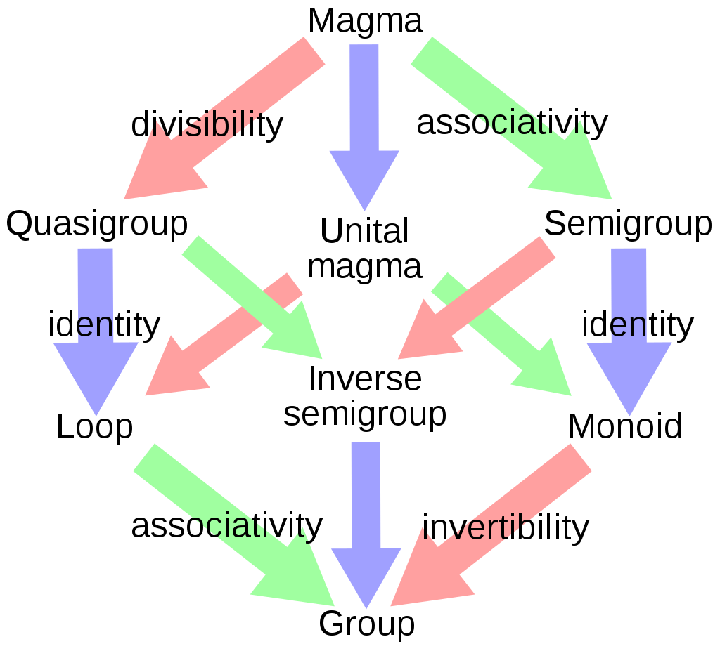
Some of the terms have transparent names and others are just weird (– hey, at least they’re not named after people! –). A magma is just a set M with a binary operation (\(b(\cdot, \cdot) : M \times M \to M \)) that maps any two elements in M to some element in M, that is, M is closed under \(b(\cdot, \cdot)\). In the words of a wise colleague, a magma is just a matrix. As more properties apply to the binary operation and M, one can go from a Magma to a Quasigroup to a Loop to a Group (and there are other paths ~). Historically, there was a lot of frustrated disagreement as everyone wanted to use the term ‘groupoid‘ for different things and about three decades later, Serre finally used the term magma.
Do we as a civilization want some of our foundational concepts to have near arbitrary names? The status quo seems to say that, yes, we do.
How is this relevant to theorem proving? I’m glad you asked.
In order to work on making E smart again, I first strip away some of E’s standard technology to render E quite a bit stupider. This is a bit like taking a group and then stripping away the assertion of associativity, identity, and invertibility before asking if we can learn how to use the group in practice anyway, without relying on these properties (perhaps re-learning them when they apply).
First, let’s cover some historical results
In the ProofWatch paper’s 5000 problem dataset, E’s auto strategy proved 1350 problems (in 10 seconds). And auto-schedule, which automagically works with an ensemble of strategies, proved 1629 problems in 10 seconds and 1744 in 50 seconds. Re-running auto-schedule, E solved 1586 (in 5 seconds) and 1785 in 50 seconds. Eh, there’s some variance.
Recall that my colleagues, Jan and Josef, did work on Hierarchical Invention of Theorem Proving Strategies, and an ensemble of these strategies proves more problems than E’s auto-schedule.
Ten of these strategies solve between 827 and 1303 / 5000 \(26\%\) individually and 1998 / 5000 \(39.9\%\) in unison.
In ProofWatch the performance was 1565 / 5000 \(31.1\%\) and 19583 / 57880 \(32.1\%\) for the best strategy with E on the Mizar data. The best 5 strategies proved 2007 / 5000 \(40\%\).
ENIGMA with feature hashing (also used in ENIGMAWatch) achieved 25562 / 57880 \(44.1\%\), and was published at ITP by my colleagues, see Hammering Mizar by Learning Clause Guidance.
ENIGMAWatch achieved 2075 / 5000 \(41.5\%\) in the paper (and 2131 / 5000 off the record) after 14 loops of training XGBoost models. Over the full dataset, off the record, 26784 / 57880 \(46.2\%\) problems were solved in 10s after 8 loops of training (10x the data helps a bit, eh?).
And while we’re at it, I hear Vampire plateaus around 27000 problems as well.
It seems going beyond this range becomes harder. I ran 15 loops of a new prototype addition to ENIGMA and it started plateauing at 2255 / 5000 \(45.1\%\).
As of 2022, we’ve predominantly switched to LightGBM because it trains faster with larger datasets and we have more freedom to change the parameters. XGBoost trains trees row-by-row to the designated depth whereas LightGBM uses a “number of trees” parameter and can in principle have very lopsided trees (with unbounded depth ;D). The histogram-based approach to finding decision points among the features may also contribute to its speed. Anecdotally, the LightGBM training seems a bit more chaotic or brittle but all we need is a good model. With LightGBM, small changes to the parameters changed its performance a lot more than the seemed to with XGBoost. ( Learning from even proofs discovered thanks to graph neural network based guidance, we’ve acquired Enigma models that can prove over 38,000 / 57,880 problems.)
Anyway, the point of these results is that: learning to guide the theorem prover works pretty well!
The improvement over these smart strategies by using gradient boosted trees are 70-170% depending on which year’s results one looks at.
We generally use the data from E with good strategies to learn how to guide a proof search even without them. – recall we do some runs 50-50 smart strategy and ENIGMA model (coop) and some runs with solely the ENIGMA model (solo). In this paper I only report solo results for two reasons: (1) they sometimes actually performed better and (2) they are even more minimal; however, sometimes I’d run coop models, too, and use their training data.
However, there are other carefully derived heuristics that help guide E to find proofs.
For example, have a glance at the favorite strategy below (mzr02):

Careful not to look deeply. The -H(…) at the end is the strategy component I described in ProofWatch, telling E how to weigh different math clauses and which ones to prioritize.
You can see there are still a bunch of options.
One of the important ones is “–prefer-initial-clauses”. This tells E to deal with all the “clauses in the problem statement” before moving on, y’know, so we don’t get lost before even reading the whole problem. The “–definitional-cnf” option determines how often clausal definitions are introduced in the process of clausification (whereby logic in normal terms is translated into universally quantified clauses).
The important one we work with here is “-tKBO6”, which refers to the Knuth-Bendix Ordering.
I actually just learned many details about this recently.
It’s related to something called the Word Problem: given two expressions and a system of rewrite rules, how do you determine if they refer to the same thing or not? This is a syntactic question. Sometimes the answer is only determined culturally and on a semantic level, such as with, say, “one-eyed wonder worm” and “heat-seeking moisture missile”.
A normal mathematical example would be “2 + 3” and “8 + (-3)”.
A semantic approach is to evaluate them: “2+3 = 5” and “8 + (-3) = 5” and “5 = 5”, so they’re equal.
In logic, we like to have clear rules to transform or rewrite, one expression into the other. This can be especially important when we don’t have a specific model in which to evaluate the expressions (and may want a derivation to hold for many possible models).
I’m not sure what these look like for arithmetic, something like: “2 + 3” = “(2 + 3 + 3) – 3” = “8 – 3” = “8 + (-3)”?
Where we may have used a rewrite rule of the form “for all a and b, a = a + b – b” to start.
It turns out in many cases this “word problem” is impossible: given Word1 and Word2, it’s impossible to say if they are the same thing or not.
One problem that can occur is endless cycles.
For example, I know that “a = b” and I start with the word “a”.
So I rewrite it “b”, and then I rewrite it again to “a”.
“a = b = a = b = a = … a = b = a = b = a”. ~ ~ ~ whee, whee, whee all the way to infinity and beyond!
Many humans are smart enough not to do this. But what if you have ten thousand words? Maybe you’ll get confused and write “a” to “b” in one place and “b” to “a” in another place?
The theorem prover E solves this problem by maintaining a global term bank that clauses are built on top of so that rewrites will be done consistently.
Wouldn’t it be good to just decide: okay, if “a = b” then let’s only turn “b”s into “a”s because “a” comes first!
That’s exactly what our smart theoretical computer scientists did in the 70s, 80s, and 90s!
They call it a Rewrite Order.
You say “x” < “x + 0”, so you can only simplify your arithmetic statements. Oops, I guess I violated this ordering in my arithmetical rewriting above!
There’s an example in group theory with the KBO (Knuth Bendix Order) on the word problem page and the same example in E’s notation on the KBO page. (Warning: for the mathematically inclined reader.)
Generally, E relies on KBO (or LPO) ordering to ensure that its proof-search is complete, namely E only finishes if it finds a proof or processes every single clause (which means there is no contradiction).
Without ordering, I believe E could terminate even if there is a contradiction in the problem and axioms (see Selecting the Selection for an example).
Recall that we write clauses “a or not b” as \(a \vee \neg b\) (such as “he’s a donkey or he’s not an ass”.)
“a” and “b” are called literals.
E works with Resolution, which is like a generalization of Modus Ponens, which says:
\((p \wedge (p \to q)) \to q\), or in words, if p is “man(X)”, q is “mortal(X)”, and X is “you”, then this says, “If you are a man and if being a man implies being mortal, then you are mortal.
In classical logic \(p \to q\) is written \(\neg p \vee q\). Either p is not true or q is true. If p is true, then “p is not true” is not true, so we know that q is true. Whereas if p is false, then we know nothing about q from this statement. This is the beauty of the material conditional: it only says something when the antecedent (p) is true. Thus “\(False \to Anything\)” is always a true statement!
The basic idea of resolution is visually very simple: you just match \(p\) and \(\neg p\) and they cancel out (because one must be true and the other false, so you’re left with the rest of the options). So one can resolve \(a \vee p\) with \(\neg p \vee b\) into \(a \vee b\).
The other way E uses KBO ordering is for literal selection (see Selecting the Selection again).
I believe in ProofWatch I said that when E chooses a given clause it does “all possible inferences” with every clause in the processed clause set.
Now you can guess that E uses the ordering to limit what is a “possible inference”.
Take the following example where we know “a and b imply c”, “a”, and “b”. We want to derive the conclusion, “c”. First De Morgan’s Law is used to represent the implication clausally as \(\neg a \vee \neg b \vee c\).
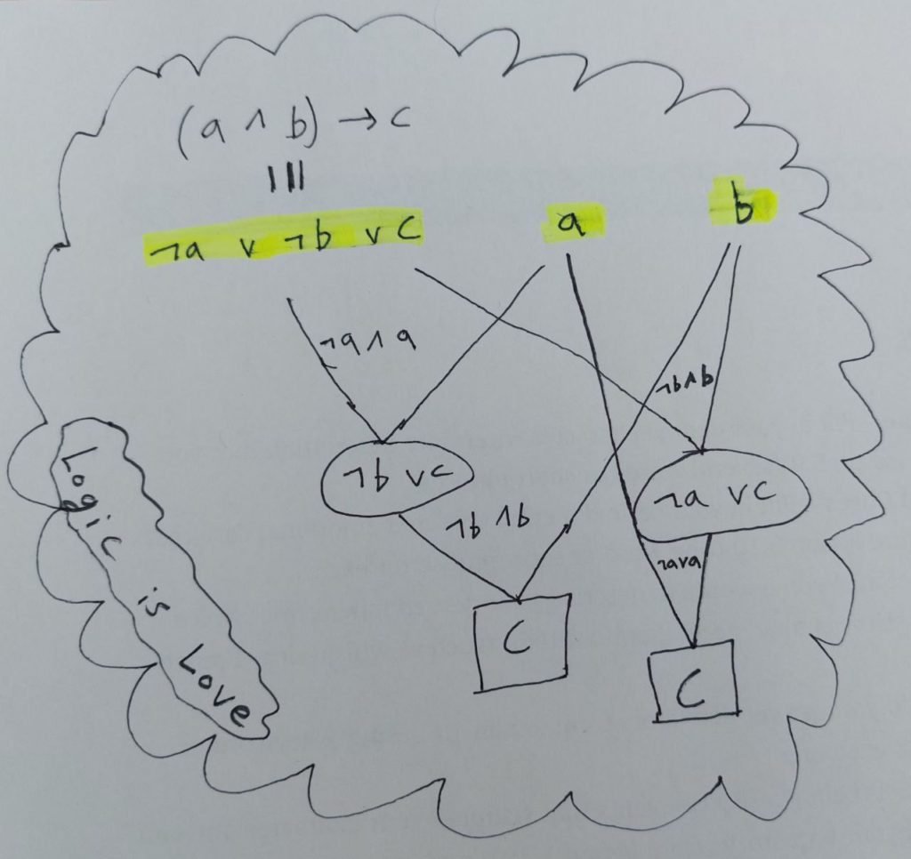
- We need to resolve with both “\(a\) and \(\neg a\)” and “\(b\) and \(\neg b\)”.
- The order doesn’t matter, so there are two maths to derive “c”.
Ideally, E won’t generate both \(\neg b \vee c\) and \(\neg a \vee c\), and in the case that E has 10,000 clauses, this could become more confusing. Moreover, as with ordering, there are cases where selecting the wrong literals may violate completion.
It seems the general strategy is to select negative literals (like \(\neg a\)) or maximal literals (according to some ordering).
So E’s not actually that free to proceed through the dark forest of first-order clauses looking for the elusive empty set \(\{\}\).
E has to look in a very systematic order to not get lost.
But that was before E had ENIGMA and her machine learning guidance!
Maybe we can learn to guide E through all the nefarious pit-falls without the limitations of adhering to KBO ordering and literal selection!
Enter our basic strategy:
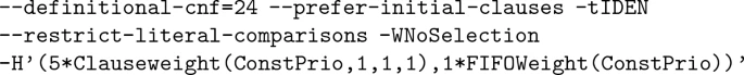
We replaced “-tKBO6” with “tIDEN”, an identity relation that says “either a = b or a and b are incomparable”.
And we tell E not to do literal selection.
The idea is to free E to be simple and naive, generating clauses without regard for order or literal selection. Normally this would confuse E, making the proof-search harder (perhaps even non-terminating, lost in some endless loop).
Thus our hero machine learning comes to the rescue and saves E from the mess and deluge of randomly generated clauses!
There are about 20 inference rules that E can use to generate new clauses. Two of these are for term-rewriting.
The way E is implemented, E cannot perform rewriting steps unless there is a clear order (i.e. only write \(a \to b\) or only write \(b \to a\)).
Even if \(a = b\), the ordering says they are incomparable (or structurally equal).
This means our E has to solve problems using resolution/superposition instead, which is probably less efficient. Rewriting can be done globally, that is, all “a”s can be rewritten into “b”s once and for all.
Is this not a metaphor for chasing utopias? Seeking greater freedom we have ended up with a draconian restriction! FUck, you suck, asshole, cocks.
Bad news:
- E is a bit stupider than desired.
Good news:
- Slowing down might limit the effects of a bad choice.
- E learned to perform pretty decently anyway.
The Experiments
Part 1: Hyperparameter Tuning
Below is what an XGBoost tree looks like.
To evaluate a clause, first, it asks if less than 19% of watchlist number 194 has been seen on the proof search. If yes, go down, and if not, go to the right. Eventually, the bottom (a leaf-node) of the tree is reached that says whether the clause is good or bad (positive or negative).
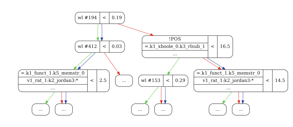
To make the evaluation more robust, we go from a decision tree to a decision forest: we learn 200 trees and add up their conclusion.
The XGBoost website has a cute tutorial on how these tree models work.
One of the main parameters is the Depth of the trees, that is, how deep are they?
A small tree of depth 2 can only split clauses into 4 different groups, asking 3 yes-or-no questions.
A tree of depth 20, like in 20 questions can split clauses into 1 million different groups (leaves of the tree).
Wow. No wonder 20 questions can normally be won – who of us even knows 1 million words?
The problem with having a really big tree is that we want to prove new problems, so if we just learn to prove the same things perfectly, it doesn’t help much.
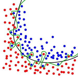
Small trees probably help to generalize better, and we call it overfitting when the model is too particular to specific examples. The VC dimension measures how many distinct data points can be distinguished by a model — if the number is high enough, any data set can be perfectly captured. The green line below is a classic example of overfitting:
Basically, don’t be “too nitpicky”.
The other main parameter is the number of Trees.
The trade-offs are similar to the tree depth. Don’t make too many or too few.
(Is the near-tautological Taoist concept of finding and maintaining balance the key to everything after all?!)
In most of the ENIGMAWatch experiments, we learned 200 trees of depth 9.
It’s not published, but we tried a bunch of different parameters with LightGBM, another gradient boosted decision tree framework.
XGBoost also lets me make trees of depth 768, whereas LightGBM has a small “leaf node limit” in comparison.
Anyway, one of the first experiments done with Basic E (our frontal lobotomized E) is to play with different settings of (Depth, Trees) when training XGBoost.
Recall that we train over many loops:
- Run E
- Train model 0 on all preceding data
- Run E with model 0
- Train model 1 on all preceding data
- Run E with model 1
- Train model 2 on all preceding data
- …
This should be especially important now that the Basic E’s performance is much lower than before (the smart strategies are about 3-4 times as good). The lobotomized version of E, basic E, will be called E0. On the 57880 problem dataset, E0 proves 3872 problems whereas two normal strategies, E1 and E2, solve 14526 and 12788 problems. Whew.
To an extent, the learning appears to be quite incremental. E learns problems in class A, then B, then C, then D, then E. Step by step.
Does it help to change the (Depth, Trees) of the models as we get more and more data? – Probably.
This is what we want to test.
We do this on a small dataset of 2000 randomly chosen problems from Mizar.
The simple, constant protocols are to use the same model for each loop of training: 100 trees of depth 5 (5,100), 100 trees of depth 9 (9,100), (13,200), (16,100), and many more that just cluttered up the graph!
I like fiddling with the parameters in a 適当 manner, using my intuition to update them as I see fit. Does it help to let XGBoost overfit a bit and then underfit a bit?
Systematic strategies feel so restrictive!
But scientists (aka conference reviewers) like things to be systematic, so I ran some of these too.
The exemplary options follow where D = Depth, T = Trees, ‘inc’ stands for incremental, and ‘dec’ stands for decremental:
- Inc: keep T fixed at 100 and step D from 3 to 33. (\(S_{[3,33],100}\))
- 32_inc: keep D fixed at 32 and step T from 50 to 250. (\(S_{32,[50,250]}\))
- Inc2: like Inc with T gradually, intuitviely decreased from 150 to 50. (\(S_{[33,3, *}\))
- Inc3: like Inc with systematic steps of T from 50 to 250. (\(S_{[3,33],[50,250]}\))
- Dec3: like Inc, stepping D from 3 to 33 while decreasing T from 250 to 50. (\(S_{[3,33],[250, 50]}\))
I’ve plotted these with E0 as a baseline over 16 loops of training.
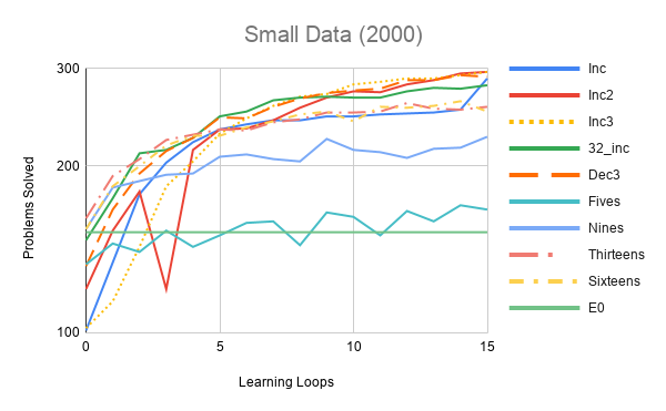
Clearly larger trees are important. A tree of depth 5 can make 32 (\(2^{32}\)) feature-based distinctions so 100 of them could do at most 3200 feature-based distinctions, which may not be much if thousands of clauses need to be judged for each problem. Go figure this doesn’t do much better than the baseline. The 51,200 distinctions of the depth 9 tree modes are much better. Depth 13 takes us to 800 thousand and the performance started dropping off by depth 32.
Inc2 and Inc3 have the smoothest performance, however, Inc actually solves one more problem than them in the last loop. Inc solves 299 whereas E0 solves 152, so performance is almost doubled 😎.
Dec3 seems to perform fine. If the final number of trees were 100 instead of 50, I wonder if it’d have kept pace with the others. Also, my casual tweaking of the parameters doesn’t seem to help much over the systematic version, tehe.
One conclusion is that while gradually changing the parameters seems fairly important, the precise scheme does not seem to matter that much. Frankly, even just getting the parameters right takes one much of the way there (such as going with Sixteens).
Next, I do some experiments on the full dataset of 57880 problems. In some cases, these models started to take 15 hours to train (yikes!). These runs are far more chaotic and I started the first looping experiments at the same time as doing the small data, so the presented order is only approximately correct.
- First I tried using a strong ENIGMA model Jan trained (proving 25562 problems). This was the first thing I tried. Initially, the model proved only 2420, less than E0’s 3872. It then does a decent job, reaching 7842 in loop 10 (just barely double E0, performance similar to in the 2000 dataset). However, the performance then started decreasing, so it was time for the second experiment.
- This time I tried gradually incrementing the model size similar to in Inc3 (with some curious perturbations). I tried doubling the feature size to 65536 (\(2^{16}\)) as well. I used data from strategies E1 and E2 to seed the learning for loops 0 to 4 and then stopped, figuring the information has been carried over and trying to learn to follow the proofs with term ordering might be confusing.
By loop 11 this surpassed Experiment 1, which seems fair as the ENIGMA model is much stronger than E1 or E2. The performance drop occurs when I decided to try 300 trees of depth 9, whoops 🤭. The rate of improvement is really slow but never quite stops.
How bad is this? If we actually got 100 new problems every 12 hours of training, after 240 days, we’d have proven all of Mizar. Unfortunately, the RAM on our servers grows slowly, the training time increases fairly quickly, and the rate of solving new problems is decreasing. - By now, I’d decided to be more systematic and just used Inc3 to set parameters. Now that I saw that boosted learning works, I wanted to try straight-up learning from E0 alone. Also, GPU training should be faster and required the feature size to be reduced to 256 (\(2^8\)).
To my surprise, this skyrocketed past Experiments 1 and 2 before the performance began dropping. The smaller feature size probably helps with the learning (and perhaps even abstractions). I suspect this could be due to overfitting as increasingly large portions of the data will consist of increasingly refined proofs of the same problems. The noise of being guided by stronger strategies from different settings may render the proofs less regular and harder to overfit. Maybe the limit of what can be done via 256 features to split trees on was also being reached? - Seeing that the small feature size helped, I repeated the setup with the addition of E1 and E2 training data up to loop 4. This seems to effectively kickstart Enigma 0 to solving 13805 problems, more than E2. Mission accomplished. Now we can officially say that Enigma can learn to guide E without term ordering.
The slope, however, looks like an S-curve that is plateauing. - Experiment 5 is pretty crazy. I went wild trying all sorts of fun ideas as to how to feed Enigma nourishing data. I’m not sure how to fairly compare it to any of the other experiments beyond seeing it as my attempt to see how far I can push Enigma Zero.
- For starters, I took strategies E1 to E12 and trained Enigma models for 10 loops as in Experiment 4 (on a small training dataset).
- I also trained Enigma models E using KBO ordering (and no literal selection) and KBO ordering (and restricted literal comparisons). The motivation is that these may serve as a bridge between standard E and basic E0.
- To create training data for the next round of meta-looping, I used data from loop 4 (the final one with data of E1-E12) and data from loop 10. This way Enigma should get abundant diverse data rather than being overwhelmed with 10000 versions of the same problems.
- Using this data, Enigma studied for 10 more loops, proving 9579 problems.
- Then I combined this with data from a loop 3 Enigma model trained with E1 (proving 21542 problems) to boost E0 in Experiment 5
- I experiment with trees of depth 512 and 1000, interleaving in depth 32 trees for variety of training data. There’s a parameter that limits how fine-tuned trees can be: min_data_in_leaf. The default is 20, so once 20 clauses are isolated, that’s a leaf of the tree.
- Curiously, 2 trees of depth 512 suffice to prove 5899 problems in loop 1. There seems to be a trade-off between tree size and the number of trees. By the end, the best results were attained with only 32 trees of at most depth 100 (which should already allow for over \(10%{31}\) distinctions).
- Eventually, the feature size had to be lowered to fit the training process on RAM.
- After 11 loops, Enigma Zero proved 15990 problems, surpassing E1 as well.
In conclusion, Enigma Zero can 4x E Zero’s performance.
This is pretty fucking cool and shows that there is some potential in guiding E or other theorem provers without these theoretical tools (such as term ordering, literal selection, hand-crafted strategy building blocks, etc).
However, the degree of training and negative data required seems to indicate that the performance will likely just be worse than that of E with KBO and literal selection. Should we just keep trying from the ground up and include more general learning of fixed strategies, ordering, et cetera? Perhaps. I am also curious to what extent the graph neural network based Enigma could help E0. Maybe if we stick with E0, we’ll find different ways to structure the learning and boosting data to make up for the increased difficulty of the search space without term ordering. [So far, however, we’ve simply moved on 😛.]
In contrast, Enigma with E1 easily learns to be far better than an ensemble of 12 (or more) strong E strategies that have themselves been machine learned.
Part 2: Responsible Parents
I’m really glad that I took notes on some contemporaneous experiments that didn’t make the 5-page short paper. When there are deadlines and lots of messy experiments, fitting everything into a short paper is difficult.
I really wanted to give ENIGMA more information about the clauses it’s evaluating. Humans are free to look at anything when trying to solve a problem, so why should Enigma be able to figure everything out only based on the conjecture features, the clause features, proofvector features, and perhaps theory features?
Thus I hacked E and ENIGMA to include the features of a clause’s parents in the feature vector.
The feature vector now includes features from the “problem statement”, the “clause being evaluated”, and the “two parents of the clause being evaluated”.
So if a clause is mapped into a vector of size 256, the full vector is of size 1024 (256*4).
The idea is that sometimes it might be easier to tell a bad seed from the parents than to look at the poor sob directly. >:D >:D >:D
This version seems to perform slightly better than the original. Yet not quite enough better to warrant writing a longer paper at the time (as if there was time, lol).
I also experiment with more extensive boosting, both of which are incorporated in Experiment 5:
- One option is to train a model on data from strategies E1 to E10 and then use this data to boost training with E0.
- Another option is to train a strong ENIGMA model with E1 and then use its data alone to boost E0.
These options both resemble Instructional Scaffolding in a way as well as the concept of a Zone of Proximal Development where a learner can do more with guidance than without, thus learning faster.

The model receives guidance on what clauses are good and learns from them.
But the model can’t just copy the notes exactly, because they rely on clause ordering.
Now there are many pitfalls that ENIGMA has to learn to help E0 avoid.
This means that with boosting, XGBoost shouldn’t be able to overfit as effectively.
Thus I tried increasing the Depth of trees to 256, 512, and 768.
It seems both options #1 and #2 work pretty well.
I ran #1 over the 5000 problem dataset (with trees ranging from depth 9 to depth 768, and the number of trees decreasing from 220 to 16).
It achieved 1679 / 5000 (33.5%).
I ran #2 on the full dataset with a weird protocol using trees of depth 512, 1000, 32, and 100. Anyway, pushing beyond Experiment 5, I found evidence E0 can be boosted to 16242 / 57880 (28%) of the problems (and looking at the results on the 5000 dataset, probably more with patience).
Looking back, I’m unsure to what extent these 16k results are thanks to the responsible parents’ features (as well as why they didn’t make the cut to be included in the paper).
Ablation Study
So far we’ve concluded ENIGMA can learn pretty well, from 361 to 1679, if given good training data.
And it’s not so bad even without boosting data: from 344 to 780 is a 2.26x increase, whereas ENIGMA only takes E1 from 1258 to 2115 in 5 loops of training. (On a 5000 problem dataset.)
However, it seems ENIGMA cannot presently make the ordering and literal selection obsolete.
How important is ordering?
How important is literal selection?
Does it have to be a good ordering?
Or can we use an empty LPO ordering (that only orders sub/super terms, that is f(f(0)) > f(0) > (0), but 0 and 1 are incomparable)? This is called Lexicographic Path Ordering.
This is called an Ablation Study: we set out to figure out how important each component is.
To this end, I ran an experiment with various options.
Note that by default E doesn’t use literal selection.
-S uses a fancy selection heuristic: -WSelectMaxLComplexAvoidPosPred
-r means –restrict-literal-comparisons is used
-L means the empty LPO4 ordering is used
-K means that KBO6 is used
The option “-r” says it restricts literal comparisons for paramodulation, equality resolution, and factoring. In practice, this seems to be almost the same as not using literal selection but perhaps a bit harsher. For future experiments with minimalistic E, one probably doesn’t need to bother using it.
First I ran each mode on its own. Curiously, literal selection with only the IDENtity order is worse than nothing. LPO helps a bit and KBO helps quite a lot. The selected literal selection strategy is actually quite good (and there are far less effective ones available in E). The Clause Evaluation Functions of mzr02 (E1) help a lot beyond KBO+S.
- 332 basic-S
- 332 basic-S2
- 334 basic-Sr
- 344 basic-r
- 346 basic1
- 376 basic-Lr
- 396 basic-L
- 415 basic-LS
- 729 basic-K
- 951 basic-KS
- 1258 mzr02
Below are the results after 5 loops of training:
- 764 Enigma+VHSLCXRh+mizar40_5k+basic-r
- 781 Enigma+VHSLCXRh+mizar40_5k+basic1
- 788 Enigma+VHSLCXRh+mizar40_5k+basic-S
- 789 Enigma+VHSLCXRh+mizar40_5k+basic-Sr
- 792 Enigma+VHSLCXRh+mizar40_5k+basic-S2
- 897 Enigma+VHSLCXRh+mizar40_5k+basic-Lr
- 934 Enigma+VHSLCXRh+mizar40_5k+basic-L
- 985 Enigma+VHSLCXRh+mizar40_5k+basic-LS
- 1265 Enigma+VHSLCXRh+mizar40_5k+basic-K
- 1708 Enigma+VHSLCXRh+mizar40_5k+basic-KS
- 2104 Enigma+VHSLCXRh+mizar40_5k+mzr02
Literal selection is still meaningless without a good ordering (which I believe is obvious from the theoretical schematic and the code). Good 😋.
The empty LPO ordering clearly outperforms the IDENtity relation and is arguably minimalistic enough to not worry about.
Curiously, the difference between KBO and LPO are almost identical before and after 5 loops of training — are there simply 333 problems that KBO helps E to solve and Enigma training figured out 2 of them?
The results with term ordering and literal selection are more interesting. The learning helps more. The gap between KS and LS increases from 536 to 723 problems. The difference between KS and K also increases by 187 problems. The largest leap in the capacity to learn seems to be when S is added to K.
While the gap between mzr02 and KS is not as big, Enigma still learns 89 problems more in 5 loops with mzr02 than with KS.
Multiplicatively speaking, the performance jumps 138% in 5 loops with Lr, which is the highest.
So to some extent, these results could be explained by the fact that the stronger methods have more training data to learn from and thus perform even better. However, ordering and selection strategies limit what Enigma needs to learn while making the proof-search easier, so I would not be surprised if learning is actually easier in these cases.
This might be a good argument for using every tool at our disposal rather than stubbornly sticking to simple settings.
As diversity is strength, I am curious whether minimal E approaches can yield some new proofs or data for the full-on E models.
As a conclusion, I think these ablation studies with Enigma and E Zero make for an interesting proof of concept.