EnigmaWatch II

I’d like to have personalized blog post versions of all of my research papers, which would ideally be done in sync, yet this is coming out 3 years later. For the next paper, Make E Smart Again, I wrote a draft of the blog post at the same time as the paper. I found that expressing the ideas in my own words before concerning myself with officialese to be helpful. Presently, I’m curating my Ph.D. thesis and find updating the blog posts to be synergetically inspiring. Please forgive me if the prose is less didactically clear than in the prior posts.

My previous post, EnigmaWatch I, explains the idea of combining symbolic and statistical learning and analyses experiments on a small dataset of 252 Mizar math problems, which couldn’t be extended due to computational slowdowns. Jan (pronounced ‘yan’) and I did some help EnigmaWatch to be run over the full 57,880 Mizar problems and the system speeds up learning over plain Enigma. You can read the full paper on arXiv: ENIGMAWatch: ProofWatch Meets ENIGMA. You can view the slides here. Or read on for an executive summary.

Why was EnigmaWatch so slow?

1. Enigma used the XGBoost framework for learning an ensemble of decision trees to predict which clauses to select next. This experimentally slowed down when the feature vectors grew over roughly 100,000 features long but training data over the whole Mizar Mathematical Library easily produced over one million features. The more mathematical symbols and combinations of them there are, the more features there will be.
2. ProofWatch needs to check whether every single generated clause subsumes a clause on the watchlist. The number of generated clauses grows quadratically with the number of steps in the proof search (because each selected clause can in principle mate with all already processed clauses). This slowed down to a crawl beyond watchlists containing 4000 clauses.

Clause Feature Hashing

To speed up Enigma’s learning, the goal is to reduce the length of the feature vectors (which is a concatenation of clause and conjecture vectors). Previously, the features in a training dataset were just numbered from \(1\) to \(N\). Now we want to do something smarter to significantly reduce the size. There are theoretical techniques for dimensionality reduction such as Principal Component Analysis that try to preserve meaningful properties of the data. These can, however, be costly. Often it’s better to just find a fast way to map the data into a small number of bins. This is called a hash function, for example, Wikipedia’s image of a hash function mapping names into numbers:

One wants the hash function to have few collisions over one’s data as well as for the values to be uniformly distributed. It’s common to incorporate random seed numbers into the hash function, too. They often work well enough 🥳.

The hash function we use is called SDBM and I’ve pasted code from The Algorithm’s GitHub:

def sdbm(plain_text: str, base: int) -> int:
      hash = 0
      for plain_chr in plain_text:
          hash = ord(plain_chr) + (hash << 6) + (hash << 16) - hash
      return hash % base

To understand the code, you first need to parse the bit shift operator. Numbers are represented in binary, that is, only with 0s and 1s. Shifting all bits left by one and adding a zero to the right will multiply a number by two. This can be faster than general multiplication implementations. In general, \(a << b\) will multiply a by \(2^b\). The function ord returns the ASCII number of a character (which is 108 for ‘l’). Let’s look at the example of hashing ‘love’ with a hash base of 69:

1. hash = 108 + 0 + 0 – 0 –> 108
2. hash = 111 + 6912 + 7077888 – 108 –> 7084803
3. hash = 118 + 453427392 + 464309649408 – 7084803 –> 464755992115
4. hash = 101 + 29744383495360 + 30458248699248640 – 464755992115 –> 30487528326751986
5. hash = 30487528326751986 % 69 –> 0

And it turns out that \(69 * 441848236619594 = 30487528326751986\). Colour me surprised!

As you can see, this sdbm function jiggles the numbers around a lot. The hash base is handled via modular arithmetic, which can be thought of as wrapping the number line around a lock so that each number becomes one between \(1\) and \(12\). Let’s see two more:

• sdbm(“(=,f,g)”, 69) = 33
• sdbm(“(f, *, *)”, 69) = 8

If you’re curious, you can see the actual code in E for hashing feature vectors and the paper first experimenting with the hash function for Enigma features: ENIGMA-NG: Efficient Neural and Gradient-Boosted Inference Guidance for E. They tested hash bases from 1000 to 32000. The smaller hash bases led to better accuracy on the training data but the gold standard benchmark is the ATP performance: does the automated theorem prover, E, prove more theorems? — no, but E didn’t prove many fewer either.

The feature vector hashing could sometimes confuse the learning algorithm, especially if two important features collide in the same bucket. Counter-intuitively, the hash function could get lucky and grouping some features might make learning easier or generalize better!

Multi-Index Subsumption Indexing

A subsumption index is a tree-based data structure that uses clause properties to help with checking whether a clause \(C\) subsumes any clause \(D\) in the index. For example, a clause \(father(zar) \vee hero(zar)\) cannot subsume \(hero(zar)\) because the number of literals are different (i.e., 2 > 1). As a brief reminder, the following subsumption holds: \(hero(X) \sqsubseteq father(zar) \vee hero(zar) \) (with the substitution \(X := zar\)).

Stephan Schulz implemented feature-vector indexing for subsumption in E^s. based on clause features that will reflect the subsumption relation (that is, \(f(C) < f(d) \iff C \subseteq D\)). The index is not perfect so a proper subsumption check still needs to be done on the clauses that are returned. There are two common subsumption queries:

1. Forward subsumption looks for a clause C in a clause set S that subsumes a given clause G.
   • E wants a clause \(C \in S\), such that \(C \subseteq G\).
2. Backward subsumption looks for all clauses C in S that are subsumed by by a given clause G.
   1. E wants the set, \(\{C \in S | G \subseteq C \} \).

For ProofWatch, backward: E wants all watchlist clauses that are subsumed by a generated clause to see if it should be prioritized.

Jan noticed that in general, C can only subsume D if the top-level predicate symbols match. The predicate symbols in these examples are “father” and “hero”. “Sister” in the following example is not a top-level predicate symbol: \(hero(sister(zar))\). Also, \(\neg hero(X)\) cannot subsume \(hero(luke)\) because it’s negated. Therefore we can make a separate subsumption index for each code, which is the set of top-level predicate symbols and their signs (+ or -).

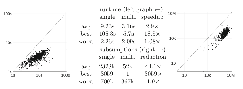
How much does this help? To find out, we chose 1000 problems at random and ran them for 1000 generated clauses (so that the watchlist of 60,000 clauses will be checked 1000 times). On average multi-index subsumption was 2.9 times faster and did 44 times fewer subsumption checks, which is pretty helpful.

Proof Vector Construction

Even with the 3x speed-up thanks to multi-index subsumption, it’s still too slow to load tens of thousands of proofs onto watchlists, so we wished to find a smart way to select only a handful of proofs to judiciously guide EnigmaWatch through proof-space.

What does it mean for a proof (a list of clauses) to be helpful? First, some of the clauses need to be matched during the proof search, otherwise, it provides no information. If I want to develop a model that helps with proving many conjectures in a corpus, a proof that provides different information for different proofs might be helpful. The ideal desire is for a collection of proofs and how much they’ve been matched to provide information about where the prover, E, is in a mathematical space (and where it should go next). A true ideal is for the vectors to form a semantic basis over the proof space, however, we talked about the easier, pragmatic question here.

To experiment with proof vector construction, I need to gather data. Strong strategy A (the same as in the ProofWatch work) proves 14822 problems, so I loaded all of these into E as watchlists and then ran ProofWatch (with strategy A) again on the full dataset of 57,880 problems. This produces a 3-dimensional matrix: [problem, given clause, proof-state vector]. That is, for each problem E outputs a list of given clauses (chosen to do inference with), whether it is part of the proof (i.e., ‘pos’ or ‘neg’), and the proof-state vector counting how many clauses on each watchlist were subsumed at this point (so that we know where E was in the ‘proof-space’ when it selected this clause). I further simplified the data by calculating the average proof-state vector for each problem to produce M: [problem, mean proof-state vector].

I experimented with four ways to construct a proof vector from this data.

1. Mean: do it again! Average the average proof-state vector over all problems this time and take the top k.
2. Correlation: Take a relatively uncorrelated set of k proofs (via the Pearson correlation matrix).
3. Variance: Take the k proofs with the highest variance (of means) across the problems.
4. Random: Just randomly select k proofs 😎

I initially set \(k := 512\). The motivation behind mean is that the proofs that are matched the most on average may be informative; however, what if the proofs resemble each other? This is the motivation to look for a set of uncorrelated proofs. Maybe a proof that is matched a lot in some problems and not much in others is more informative, thus is the incentive to try selection by variance. And maybe statistical methods will be biased more than just randomly sampling proofs :-D.

That’s about it. Let’s see how the results look ;- )

Performance

• As usual, testing is done on 5000 random Mizar problems.
• E runs are done with time limits of 60 seconds or 30,000 generated clauses.
  • This is approximately the average number of clauses the baseline strategy generates in 10 seconds.
• The first curiosity is how the proof-vector construction performs on its own:

• Yay ~
• A 15% improvement by Mean is considered pretty decent.
• From this data, I performed some training loops:
  1. Train a model for loop k.
  2. Run EnigmaWatch.
  3. Gather all the cumulative data.
  4. Goto step 1.

• Mean EnigmaWatch proves 55% more problems than Mean Proofwatch
  • And 71% more than the baseline strong E strategy.
• That’s pretty fucking rad. Machine learning works. Glory be to the machine progeny of mankind!
• At a glance, the proof-vector construction method doesn’t matter much.
• Furthermore, while EnigmaWatch performs 8.8% better than Enigma in loop 1, by loop 4 they’re all plateauing to the same value.
• They provide ample complementary, proving almost double the baseline strategy!
  • Which is unfair as in ProofWatch, we saw 5 strong strategies prove 1910 problems (on a different set of 5000 randomly selected problems), which would only make a 16.6% boost.
  • Yet, hey, all of these models work with the same baseline strategy with 50-50 cooperation.
  • One observation of mine is that it’s really hard to make ‘fair’ performance comparisons in ML.
• The results clearly plateau: even running vanilla ENIGMA and Mean for 14 loops, the results aren’t much better and the complementarity is not wavering:

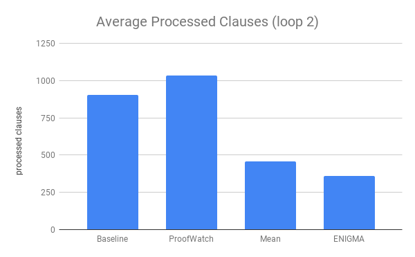
• Using the watchlist seems to result in processing more clauses on the road to a proof (probably because of false positives and the way that anything matching a watchlist is prioritized no matter the weight assigned by another strategy or ML model).
• Enigma reduces the length of the prof search by more than half.
  • Looking back, I’d be interested to look at the number of processed clauses divided by the length of the proof found. To what expect in Enigma memorizing the proofs? And to what extent are these smart heuristics?

• A surprising result is that EnigmaWatch trains twice as fast as Enigma in the later loops:

• This is really cool as, in later experiments with Enigma, I’ve ended up spending 12+ hours on training.
• I believe one reason for this is that the watchlist features help to quickly split the clauses into positive and negative.
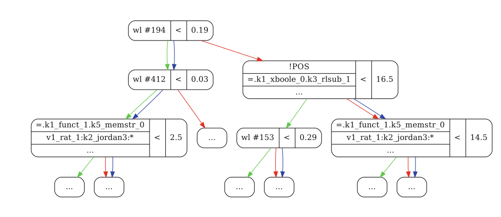
• In XGBoost decision trees, a red arrow means ‘no’, green means ‘yes’, and blue means the feature isn’t present. XGBoost decides which feature to use in a greedy manner based on how well it splits the data.
• In the example below, the most discriminating feature was whether watchlist #194 was 19% matched or not.
  • One hypothesis, having not inspected carefully, is that the initial processing of theory clauses for some problems will match watchlist #194 more than 19%, so that this allows Enigma to know what sort of problems it’s dealing with.
• I’d speculate that the informative value of watchlist features could grow as more of the proof-data is generated using the watchlist: could the attempt to create a proof-state characterization be a self-fulfilling prophecy?

Post Publication Experiments

I did some additional experiments learning on the full Mizar 40 dataset after the publication. Some of the most fun, wild experiments I do come in a burst after submitting a paper — “Yaaay, I’m finally free to just play with the tech and see what happens 🤩!” I wish I’d written this post earlier as I don’t remember what all the filename annotations mean:

knn-32-var-update_Enigma+VHSLCWh+mizar40+mzr02-wlr+10+concat-hash-32768+knn-32-var-update_loop02+mzr02-wlr+EnigmaXgbSNo

Let’s see. I was trying to do some sort of k-medoids algorithm to select among the top proofs suggested by the “variance” style of proof-vector curation, leading to 32 watchlists of proofs. “VHSLCWh” is a code for Enigma features (vertical, horizontal, symbolic, length, conjecture, watchlist, and hash — I think). Dynamic watchlist, assigning higher relevance to clauses matching watchlists that are more “completely matched” is denoted with “wlr”. Features are hashed into /(2^15/) bins. The base strategy is called “mzr02” (which is the strong strategy used in this paper). This is the 3rd loop (starting from 0). We’re using XGBoost (rather than LightGBM) and the ‘S’ in ‘SNo’ indicates that the strategy is run in the 50-50 coop mode. I tried various ways of combining top-proofs from the different proof-vector curation methods, as well.

The main conclusion I remember is that proof-vectors of sizes 32 and 64 actually seemed better than the ones of size 512 in the paper. (Gee, really, this should be publicized if anyone is going to be inspired from the paper and take some details overly literally as ‘state-of-the-art’ 🤔 😋.) Training times over 58k problems being larger and more inhibitive, I didn’t do more than 3 loops for a gain of 72% (25667 / 14960) with the above strategy and 59% for Enigma (which is worse than the 64% in 3 loops in this paper). Moreover, EnigmaWatch was run for only 10 seconds, so the “60 seconds or 30,000 generated clauses” limit wasn’t needed.

Becoming a researcher myself, I curiously note that the published results are almost always not the whole story. In my case, the hidden results are usually at least as good as the public results. Even if I get better results, they may be done in a chaotic, playful manner that is hard to concisely present. I wonder how research, its accountability, and verification could be done in a manner that allows positive and negative results to be shared with fidelity.

Concluding Remarks

The results of the EnigmaWatch experiment were intriguing to interpret. One ideal result researchers aspire for is that the new method unilaterally outperforms the ‘old’ ones, yet these experiments indicate that EnigmaWatch and Enigma perform equally well (aside from the training time of EnigmaWatch being shorter). The two approaches in these experiments plateau to different sets of roughly 2100 solved problems, with roughly 100 not shared between them. It’s not clear that this complementarity can’t be gained via training multiple Enigma models with different parameters or baseline strategies.

Is EnigmaWatch a success? Kind of.

Enigma is normally run by us in 50-50 coop with a strong E strategy yet this is not necessary. In my experience, Enigma works just fine with 100% Enigma as the sole clause evaluation function (and a constant priority function plugged in). Generally, in the experiments I’ve done (and are, I believe, mostly unpublished), the solo performance takes longer to plateau to roughly the same performance as the coop approach. Coop almost always performs marginally better (but not by much). EnigmaWatch vs EnigmaVanilla seem to have a similar relationship: EnigmaWatch starts off ahead yet the limiting performance is roughly identical. One would probably be wise to use EnigmaWatch even though both EnigmaWatch and coop Enigma are arguably unnecessary.

At present, both ProofWatch and Enigma code were updated to the latest version of E but in separate GitHub repository branches, so EnigmaWatch is history. (I will most likely remedy this in the near future.)

In hindsight, I curiously note that I only compared EnigmaWatch’s performance to Enigma’s performance in the Tableaux paper. The feature hashing had already helped Enigma to attain a 70% improvement in a concurrent publication, so my focus was on whether EnigmaWatch improved upon this. In the big picture, I was adopting a view that I’d criticized in the past when comparing chasing perfection in machine learning to the oddity that is competitive sports: why is it so important to have two of the best tennis players on the planet compete to see who is “0.000001% better”? They’re both highly skilled players. Mastery seems to be more important than competing to be the best. In the theorem proving context, this suggests the more important question is whether a method helps to prove conjectures that other methods would miss. I totally could have mentioned that Mean provides a 71% improvement over the baseline in ‘4 loops’.

Looking back, I think my tendency for intellectual humility may have struck. In the big picture, is it so important to have EnigmaWatch beat Enigma? They’re both strong players scoring around a 70% improvement with their individual strengths and weaknesses. Their combination provides an 85% improvement in 4 loops and a 95% improvement in 13 loops (vs an 82% improvement by each individually). Since then, Enigma models have reached lofty heights of at least 170% improvement (however it’s tricky to gauge as this involved learning from proofs discovered via Graph Neural Network guidance). Perhaps this number would be even higher if we’d kept EnigmaWatch up to date 😋.

Keeping the big picture in mind seems difficult when participating in a culture that values myopic comparisons of the current work against the “state-of-the-art”.

On of the core ideas of EnigmaWatch is to allow the machine-learned guidance for E to know about the proof-state. At present, the Graph Neural Network evaluates clauses in the context of the already processed clauses, which is a solid step toward context-aware proof guidance. I tried to crudely featurize the processed clauses and throw them into one amalgamized vector to give to Enigma. This “processed clause vector” would represent the proof-state. In practice, this led to very little improvement or complementarity. Proof-state representations for the guidance of automated theorem provers is an open research topic.

Next up is Make E Smart Again where I explore how far gradient boosted decision trees can go toward replacing the standard technology for proof-search guidance and management.