Parental Guidance

Parental Guidance is the fulfillment of a research question that had been nagging me since the early days of my Automated Theorem Proving (ATP) research. (See the paper and the slides.)

Let’s review how the superposition calculus based refutational theorem prover E’s respiration works. To attempt to prove a conjecture C from axioms A, E first negates C and then adds all the clauses in \(\{\neg C \cup A\}\) to the processed clause set U. E then processes the clauses in U one at a time according to the given clause loop:

1. Choose a given clause g.
2. Do inference with g and all clauses in P as possible.
3. Process the inferred, generated clauses: simplify them, remove redundancies, evaluate them, and add them to U.

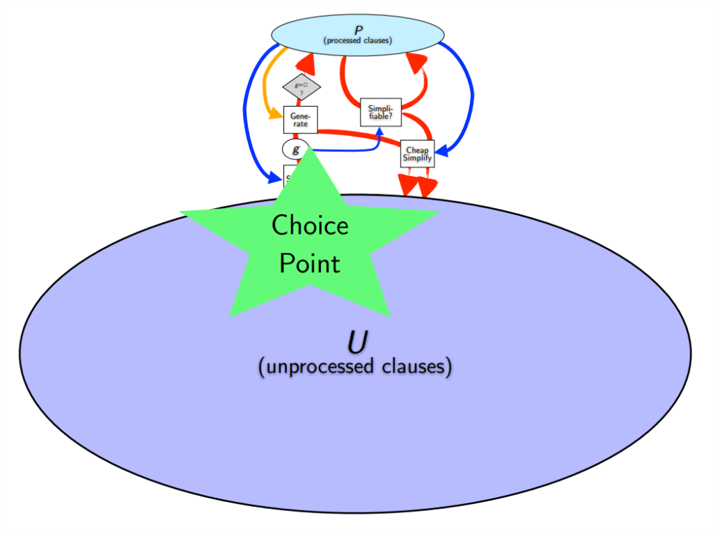
Usually, step (1) is considered the Choice Point: how can we intelligently choose what clause to do inference with next? Every clause in a proof will have to be chosen once, so getting this step right is pretty obviously important. Moreover steps (2) and (3) are both fast and there’s an important invariant that at each step all mutual inferences among processed clauses in P have been computed. The refutation completeness of the proof search is highly valued among many automated theorem proving researchers: if there is a proof, it will be found (or E will run out of resources 😛).

Yet the question was nagging me from the ProofWatch days: is it really wise to do all possible inferences? Humans don’t really do this. We rule out possible inferences that seem uninteresting (and we may not notice all possible inferences anyway, lol). Furthermore, idealized completeness is not the scenario we deal with in practice. If the theorem prover runs out of resources, then we do not know whether there’s a proof or not. E could run forever on some problems (indicating that \(\{\neg C \cup A\}\) is satisfiable). E is usually run from 1 to 300 seconds, so the real question is “completeness within 300 seconds”. I do suspect there is still value in sticking close to complete algorithms in principle.

I tried adding parent features to EnigmaWatch way back in 2019. They were concatenated onto the feature vector along with the clause features and the conjecture features (and theory features, which the axiom clauses get unified into). I noticed perhaps a 1% increase in performance on some Mizar40 experiments, which wasn’t significant enough to run with. I also tried merging all the processed clauses into one ‘feature vector’ a bit like the theory features to ‘represent the state’. This also didn’t help or hurt much. Since then, Jan Jakubuv revamped the ENIGMA code in E to be more modular so that adding new features is much easier 🥳🎉.

In 2020, I finally got around to trying to inject learning into step (2). The idea was to only let responsible parents mate to produce offspring, thus simplifying the choice of a given clause and saving time on the generation and post-processing of clauses. In doing so, a number of nuanced details surfaced, which led me to question the value of this sort of parental guidance. I can sympathize with my predecessors for not attempting to add AI to the clause mating phase.

The first issue is that to have an ML model (based on LightGBM) evaluate the compatibility and fitness of a given clause g with every clause in P will require \(|P|\) calls to the model (which is more expensive than just evaluating the generated clauses with a comparable model). Each step of the proof search will require one more evaluation call.

— Okay, then, how about only using the model to evaluate the compatibility of g with clauses in P that g can logically be mated with? Looking through E’s code, it turns out that by the time the clauses in P with which inference can be done are found, just generating the bloody children clauses is computationally trivial. E represents clauses by reference to shared term indexes and also uses these term indexes to see whether inference is possible (specifically paramodulation, which also implements resolution). So it turns out that checking whether inference can be done between clauses a and b is not much harder than just generating their children. Whoops, no wonder people haven’t bothered 😅😝.

A related issue is that when prototyping on some problems, the unprocessed clause set U would become empty (when it shouldn’t). Thus I developed the freezer set F to place generated clauses that are filtered by the parental guidance model (that judges their parents to be irresponsible 😈). This seems to practically preserve “completeness within 300 seconds”; technically the completeness of the proof search can theoretically be preserved by having a strategy that does “first in, first out” once every 10,000 clauses mixed in with the other strategies (and also assuming good term ordering and literal selection).. The clause freezing and reviving only if U empties probably violates theoretical completeness guarantees. This workaround is cool, buuuuuuut, now there is no space-saving to the filtering of clauses either 🤯🙈!

Well, shucks. The idea seemed good but when going through the code, it seems as if the inference is already so fast and low level that there’s no room for ML. There is the small benefit to skipping work simplifying the clauses (which could be lost by losing the gains of redundancy removal). Is there any conceptual redemption?

In the solo ENIGMA setting where only an ML model is used to evaluate the clauses, if a clause is evaluated with a really low score, it’ll just sit in U and practically never be selected (at least not in 15-30 seconds). However, we usually run ENIGMA in the coop setting where the ML model’s evaluation is used to select half of the given clauses, and a strong E strategy is used to select half of the given clauses. Thus no matter how bad the ML model judges a clause to be, the E strategy can boost it. This is both a feature and a bug.

The experiments I recall doing between solo and coop indicated that the solo runs will generally catch up to coop in performance and that the rate-of-learning is slower. This is similar to what I observed in EnigmaWatch II when I ran ENIGMAWatch and ENIGMA for 13 loops: ENIGMAWatch learned significantly faster in the first iterations and by loop 4 ENIGMA had caught up. ENIGMA without clause ordering and literal selection (a la Make E Smart Again) showed promise but I did not manage to support its development to the point of catching up.

I can read this two ways:

1. Maybe we should stick with the pure ML approach and just take solo as far as it can go, just as we’ve switched almost entirely to ENIGMA Anonymous where symbol names are abstracted away to functions, predicates, and their arities.
2. Maybe we should throw together everything that speeds up the learning rate: coop and proof-vectors clearly help.

And now parental guidance can be redeemed.

If we stick to coop mode, then there may be value in running E with two ML models: one for clause selection as usual and another that filters sketchy generated clauses based on their parents’ features so that neither the clause selection model nor the stronger E strategy gets to evaluate them (unless they’re unfrozen). The parental guidance model can function as a (fast) rejection pre-filter, a sort of prejudice-bot, for all the E strategies at once. This could become even more interesting if we for some reason use even more than 2 strategies together in E.

I note that this function of parental guidance could also be fulfilled by placing a filter fully after clause generation and simplification but before evaluation by other heuristics. This pre-filter could even be based on only clause features. The version implemented inserts the parental guidance filter between generation and simplification, however 🤷‍♂️😋. One hypothesis is that the clause features will be very similar to the merged features of the parent clauses. I am not absolutely sure that the location of the parental clause mating filter is optimal. The code is pretty neat if you wish to experiment with alternatives.

In 2019, I tried concatenating the parent clause feature vectors, thinking that this losslessly conveys the information to the learning algorithm. However, what if merging the feature vectors will simplify the search space (which is mostly done by adding feature counts and in some cases taking a maximum or minimum of some features). I experimentally test both \(\mathcal{P}_\textsf{cat}\) and \(\mathcal{P}_\textsf{fuse}\) (where ‘fuse’ looked better than ‘merge’ as a subscript).

For what it’s worth, LightGBM is just developing decision trees based on comparing features to numeric values. It’s difficult to simulate the difference between parent A and parent B’s features, so it could help to increase the features! Maybe we can concatenate parent A features, parent B features, merge features, and difference features. Grant the gradient boosted decision tree learning algorithm the responsibility to choose the most informative features.

The next fun question is how to generate and curate training data? Usually, we use the heuristic that any clause in a proof is a positive example and any clause that was selected but not in the proof is a negative example. Generated but not selected clauses aren’t even seen by the Clause Selection Enigma model training processes. Now the goal is to train a model that judges whether clauses should even be generated. I imagined two options:

1. \(\mathcal{P}^\textsf{proof}\): extend the usual method to classify parents of proof clauses as positive and those of all other generated clauses as negative.
2. \(\mathcal{P}^\textsf{given}\): if the training data comes from a well-trained ENIGMA model, maybe any selected clause’s parents are good enough to be considered positive and those of all unprocessed clauses can be negative?

Examining a small data-set, there are not that many overlaps in either case (and actually a larger percentage in \(\mathcal{P}^\textsf{proof}\) (2.8% vs 1.1%); anyway, if a pair of parents gave birth to both good and bad children, we generously consider them positive exemplars 😉.

For this paper, we actually split our data into train, development, and holdout sets (which are terms used to help diminish confusion between “validation and test sets“). The split is 95%-5%-5%. So the training set is 52088 problems and the other two are both 2896 problems.

In my previous experiments, the only metric was how many problems on the Mizar dataset can be proven compared to the baseline. Any increase and new problems were considered good and we didn’t particularly worry about overfitting: any model that truly overfits ‘too much’ won’t solve new problems, right? 😜.

We’ve been curating proofs to Mizar problems and have gathered proofs of 75.5% of them (43k and counting). You can see some interesting ones listed on Josef Urban’s repo. For this collection, we’ve even taken some proofs from Vampire and Deepire. This gives us 36k training problems (out of 52k) to start with. Jan trained a LightGBM model we call \(\mathcal{D}_\textsf{large}\) on this dataset, using up to 3 proofs per problem. (Ironically, the model is not very large as it consists of 150 decision trees of depth 40 with only 2048 leaves.) A baseline GNN (graph neural network) model \(\mathcal{G}_\textsf{large}\) is also trained on this large dataset of 100k proofs, which took about 15 hours.

To generate training data for parental guidance, I ran \(\mathcal{D}_\textsf{large}\) on the 52k training problems (with a 30s time limit) — this requires printing the full derivation information for all generated clauses, which takes up a lot of space compared to the usual output (and the negative examples can already take up annoyingly much space).

This is where another problem enters the picture. Initially, I had thought to co-train the clause selection and parental guidance (PG) models; however, it was turning out to be easier to get better results by keeping \(\mathcal{D}_\textsf{large}\) fixed and just training successive parental guidance models. I still believe that fundamentally, co-training should be superior but the training protocol requires more sophistication than I set up. Now the whole idea of \(\mathcal{P}^\textsf{given}\) may be confounded: for I’m telling LightGBM that a “clause that \(\mathcal{D}_\textsf{large}\) selected mistakenly is ‘good'”, so the PG model will pass this clause’s parents and \(\mathcal{D}_\textsf{large}\) will mess up again and again. The prediction is that the \(\mathcal{P}^\textsf{given}\) data curation approach will flop (unless clause selection models are also newly trained).

On the \(\mathcal{P}^\textsf{proof}\) data, there are 192 negative examples for every 1 positive example. LightGBM has a parameter to adjust for imbalanced data but it helps to actually just reduce the number of negative samples. I do this by randomly sampling negative examples on a problem-specific basis (to ensure that almost every problem will have some negative examples to represent it). This is hereby colled the pos-neg ratio \(\rho\), the positive-negative example reduction ratio.

The Experiments

For the experiments, I used a 300 problem subset of the development set to test out different models and parameters. There was not enough time to do a thorough grid search over all interesting combinations, so I performed a succession of grid searches to refine the models and parameters.

Most of the experiments are run with coop Anonymous ENIGMA, that is, the features abstract symbol names to just “function” or “predicate” and the arity (number of arguments).

The main LightGBM parameters being tuned are the number of trees, the number of leaves per tree, and the maximum depth of the trees. I believe the learning rate is fixed at \(0.15\).

The LightGBM models output a score between 0 and 1 indicating the estimate that the sample is positive. One would normally take \(\gamma=0.5\) to be the threshold value where any pair of parents rated below this have their offspring frozen; however, the penalty for false negatives is very high: if a necessary proof clause is frozen, E may be very unlikely to finish the proof in time. Every model is evaluated over the 300 problem devel set with each of these nine parental filtering thresholds: \(\gamma \in \{0.005, 0.01, 0.03, 0.05, 0.1, 0.2, 0.3, 0.4, 0.5\}\).

I decided to test the merging version \(\mathcal{P}_\textsf{fuse}\) first with both data curation methods, \(\mathcal{P}^\textsf{given}\) and \(\mathcal{P}^\textsf{proof}\). The average pos-neg ratio for \(\mathcal{P}_\textsf{fuse}^\textsf{given}\) is only 9.2, which is pretty low, so I’d predict fine-tuning the pos-neg ratio not to be significant. I tested keeping the ratio, \(\rho\), as is as well as the values \(\rho \in \{1,2,4,8,16\}\). As usual in my experiments, a lot of wonky, freaky prototyping is done before the systematic experimentation begins, which is where the LightGBM parameters come from 🐇🎩.

Aaaand, as predicted, the pos-neg-ratio doesn’t matter for \(\mathcal{P}_\textsf{fuse}^\textsf{given}\). Turns out the results are also less dependent on the threshold. And the performance is inferior (except where \(\mathcal{P}_\textsf{fuse}^\textsf{proof}\) gets bogged down by 192 negative samples per positive). Otherwise, only considering proof clause parents as positive is superior. For comparison, \(\mathcal{D}_\textsf{large}\) solves 159/300 problems, so almost every run is technically an improvement.

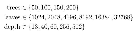
Now I can fix \(\rho=4\) to tune the LightGBM parameters. The grid search is over the following values (selected semi-arbitrarily):

This makes for 540 (3*5*4*9) evaluation runs on the small devel set. A model consisting of 100 trees with a max of depth 40 and 8192 leaves proves 171 problems with the threshold of \(\gamma = 0.05\). This model is 16 times larger than the one used to tune the pos-neg ratio. Curious to check whether this boost \(\mathcal{P}_\textsf{fuse}^\textsf{given}\), I discovered that with these parameters \(\rho=8\) and \(\gamma = 0.1\) score 163 problems — close but no cigar.

For the \(\mathcal{P}_\textsf{cat}\) experiments, I ditched the \(\mathcal{P}^\textsf{given}\) data curation method as it seemed a poor use of precious compute cycles. I also tune the pos-neg reduction ratio using the model parameters that worked best with the merge data (because they’re probably better than what I had before, right?).

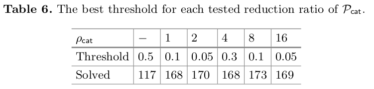
w00t! The concat method proves 2 more problems and that is with a higher threshold of \(\gamma = 0.1\). The fact that reducing negatives is apparently less important suggests the models can be more precise when parent clause features are concatenated. I initially tested \(\mathcal{P}_\textsf{cat}\) with the same parameters as \(\mathcal{P}_\textsf{fuse}\) but one of the models had a max depth of 256, on the edge of the grid search cube, so I dynamically expanded the scope of the grid search for 1080 eval runs:

The best 8 models are run on the full development set:

From the bird’s eye view, running training 120 models to improve the performance by 1% seems a bit silly, especially when the models performing best on the 300 problem devel set didn’t perform quite as well on the full development set. And while a ‘smaller’ model performed best as a ‘fast’ rejection filter, it’s still 2.6 times bigger than \(\mathcal{D}_\textsf{large}\).

What I find more compelling is the number of parametrizations that outperform the baseline (\(\mathcal{D}_\textsf{large}\)). Only 154/1080 runs perform worse and 73 do the same:

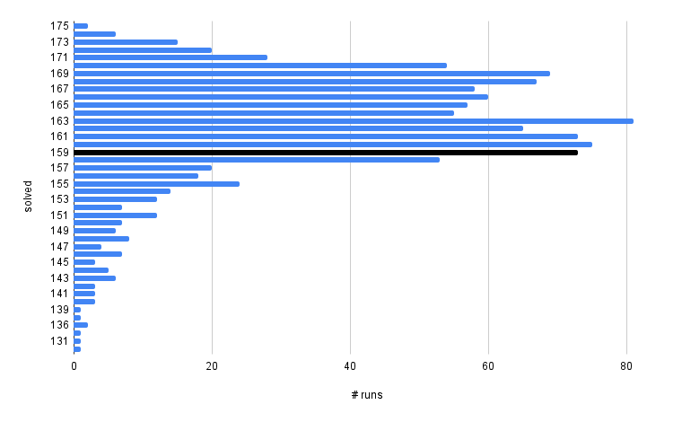
As I’ve posited before, in sports or machine learning, chasing perfection and outperforming others by a fraction of a percent can distract one from the big picture view: almost all professional sports players are fucking good. Likewise, 80% of the parametrizations tried resulted in an improvement over the baseline. It’s not hard to experience success when using parental guidance models trained on data from a strong clause selection model to support.

Curiously, larger models seem to work better with the threshold of \(\gamma = 0.05\) and smaller models seem to work better with \(\gamma = 0.2\). I would have expected the larger models to be more precise, allowing a higher cut-off. I wonder if the smaller models don’t produce as small numbers due to having less capacity to discriminate. (Ah, there are so many interesting, low-priority experiments that could be done! 🤓🥰). The crappy runs mostly consisted of thresholds, \(\gamma \in \{0.3, 0.4, 0.5\}\) and the only parameter that consistently performed sub-par is \(\gamma = 0.5\). Go figure 😋. Primarily larger models managed to make the threshold of \(\gamma = 0.5\) work, which is what I’d have expected.

Finally, I did an evaluation of the best models for different versions of parental guidance on the holdout set, too, for 30 seconds. (Small trains is a 5792 problem subset of the training set.)

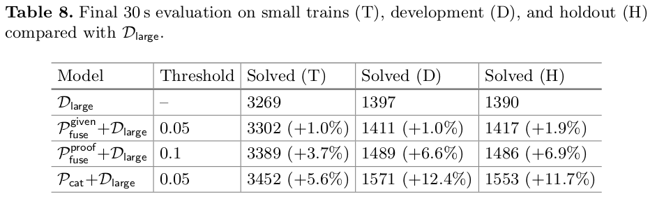
A gain of 12% is pretty good. Moreover, the gain is twice as good on the development and holdout sets than on the training set, which indicates that the training is not overfitting (as much as \(\mathcal{D}_\textsf{large}\)). The tentative conclusion is that parental guidance helps despite some reasons to doubt its efficacy.

When prototyping, I tried co-training clause selection models along with parental guidance models. The performance was about the same as just using the pre-trained (\mathcal{D}_\textsf{large}\) and the variance was higher. I also tried just using parental guidance along with a strong E strategy. This seemed to perform almost as well as just using a clause selection model but a bit worse and requiring loops of training with only its own data (as it could be confused otherwise).

---

This paper also included independent work with colleagues.

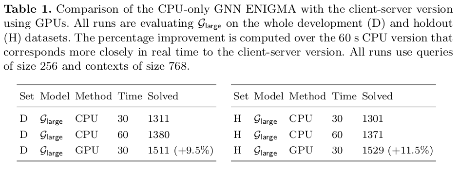
The first parallel work is the development of a GPU server to process clause evaluation queries with the graph neural network (GNN). There’s a significant startup overhead when loading the neural model onto the GPU, which can become prohibitive when running at low time limits. The new Cloud ATP Guidance System is a persistent multi-threaded GPU server that accepts JSON queries from multiple E clients and processes them in batches. This means that 160-fold parallelization is needed to saturate the CPUs on our machines (with 36 hyperthreading CPU cores) versus the only 70-fold parallelization for the CPU version because the E clients wait while the GNN is judging which clauses to select next. Running the CPU-version like this for 60 seconds per problem over the devel set took 27.5 minutes and running the GPU-version for 30 seconds per problem took 34 minutes to finish, which seems roughly fair.

Comparing the performance of CPU-only and GPU-server performance of the ENIGMA-GNN seems complicated. Sometimes we’ve used the abstract time (number of processed or generated clauses) for this purpose. In this came my colleagues chose to go with rough wall-clock time. I’ve noted before that “fair comparisons” can be a really murky, difficult concept when dabbling in machine learning (with iterated models, etc). Looking at the timed-out problems, the GPU-version generated almost 4x as many clauses in its “30 seconds” than the CPU version in 60 seconds, which indicates a hefty speed-up. The performance improvements also appear significant enough to not be a fluke. Heck, the GNN in coop with an E strategy completely trumps \(\mathcal{D}_\textsf{large}\) with parental guidance! 💻🧠🥳

The next parallel development is called “2-Phase ENIGMA.” The idea is to combine a LightGBM model and the GNN model into a single E strategy. Since the LightGBM is faster, it’ll act as a filter and score all the clauses before the GNN sees them. Clauses that don’t make the cut get assigned a very high weight (and won’t be sent to the GNN for evaluation). This way ENIGMA can make the most of the GNN’s precious GPU compute time.

To test 2-phase ENIGMA, they trained two LightGBM models, \(\mathcal{D}_\textsf{large}\) and \(\mathcal{D}_\textsf{small}\), and two GNN models, \(\mathcal{G}_\textsf{large}\), and \(\mathcal{G}_\textsf{large}\). As with the PG experiments, they did parameter tuning grid searches on 300 development problems. The parameters to tune are the filtering threshold, the number of clauses to query the GNN with at once, and how many processed clauses to include as context when querying the GNN.

To make a long story short, the improvement over the best standalone model, the GNN, was best with \(\mathcal{D}_\textsf{small} + \mathcal{G}_\textsf{small}\) (6.6-9% on the holdout set) versus \(\mathcal{D}_\textsf{large} + \mathcal{D}_\textsf{large}\) (4.8-7.3%). Probably because the small GNN is much weaker at 1277 problems versus 1529 problems. Anyway, have a table:

---

So the GPU-server, 2-phase ENIGMA, and Parental Guidance all improve ENIGMA’s performance. Pretty cool. Can we combine them further?

Right before the deadline for FroCoS, we tried training a parental guidance model based on the GNN \(\mathcal{G}_\textsf{large}\)’s runs on the training set, just feeling lucky with the same model parameters as for PG with \(\mathcal{D}_\textsf{large}\). As with the 2-phase ENIGMA experiments, grid searches are only done over the threshold, query, and context, keeping the models fixed. With a threshold of \(\gamma = 0.01\), this scored 1623 problems on the holdout set in 30 seconds, better than both PG and 2-phase results so far.

Finally, we explore a 3-phase ENIGMA with parental guidance, a pre-filter LightGBM clause selection model, and the ultimate GNN clause selection model. The 2-phase filter threshold is kept at 0.1 and the PG threshold of 0.01 is still the best. Even though the evaluation cost is higher, the performance is the best with 1632 problems solved on the holdout set, 60% higher than E’s auto-schedule and 17.4% better than \(\mathcal{D}_\textsf{large}\). Boo-yah!

Mathematically, it seems the GNN along with 3-phase ENIGMA is starting to unlock computational proofs such as the differentiation of “\(e^{\cos(x)}\)” into “\(-\sin(x) e^{\cos{x}}\)”. Doing these proofs from first principles and formal rigor in Mizar can be surprisingly hard given that it’s fairly easy to “write algorithms to do standard derivatives”. It seems juggling the soft types can be part of what makes these difficult for E. I do sometimes get suspicious: if this is so hard, perhaps there is something off with the way we’re doing it. As a related example, in the Lean theorem prover and programming language, natural numbers are represented inductively:

 Inductive nat : Type :=
   | 0 : nat
   | S : nat -> nat.

This means that 1 is “S(0)” and 10 is “S(S(S(S(S(S(S(S(S(S(0))))))))))”. Last time I checked, I believe that Lean represented numbers up to some fairly large threshold like this, in a unary number system. This is mathematically sound and simple yet computationally inefficient. I believe they have some hacks to convert these to a standard bytecode format for fast evaluation by the GNU multiple-precision library. This seems like a more practical approach than actually relying on theorem provers within an inefficient mathematical framework, but it’s still really cool that the ML guidance for E has finally begun to unlock mathematical calculations :- ).

What I really love about this work is how ENIGMA is becoming some hybrid-AI borg full of various ML models working together. When one recalls that even the “strong E strategies” were learned via AI methods and premise selection can also be done via ML such as the GNN or LightGBM, the vision of a more general AI system starts to manifest. Of course, maybe there will be additional models, weaving together efficient computational libraries with theorem proving and ML to guide its application. This seems to be what the incremental ground-up approach to aiming for general AI, AGI, might look like. Components are tested one by one, tested on benchmarks, and then their combination is also tested. I lean toward keeping the high-level vision in mind at all times and am grateful for the experience doing “obvious” groundwork.