Research Shorts: Measuring Lemmas

In math, lemmas are considered intermediate results, which is fairly pragmatic definition. Lemmas can help us to structure proofs, too. When considering a difficult theorem, it may help to conjecture a bunch of sub-goals that might be easier to prove and then to prove the main theorem from these ingredients. These are lemmas.

A good example of a simple lemma is Euclid’s Lemma, which says that if a prime number \(p\) divides a product of two numbers \(ab\) then \(p\) divides \(a\) or \(b\) (and possibly both).

As an example, take \(a = 2\) and \(b = 10\). The primes that divide \(20\) are \(2\) and \(5\), so the lemma holds as \(5\) divides \(10\) (because \(10 / 5 = 2\) is a whole number) and \(2\) divides itself evenly (as well as \(10\)). For a composite (non-prime) number, such as \(4\), while \(20 / 4 = 5\), \(4\) neither evenly divides \(2\) or \(10\) (\(a\) or \(b\)).

Euclid’s Lemma is helpful in proving the Fundamental Theorem of Algebra (also known as the Unique Factorization Theorem and the Prime Factorization Theorem). The theorem is really cool in my opinion! The statement is that every integer greater than \(1\) can be uniquely represented as a product of prime numbers. For example, \(20 = 2*2*5 = 2^2*5\), \(69 = 2*23\), \(666 = 2*3^2*37\), \(1200 = 2^4*3*5\), and \(1337 = 7*191\).

I liked the explanation given in The Joy of X. Begin with the intuition of the multiplication table. Any number can be represented by a line of single units by counting. Every composite can be counted in squares and rectangles as well, such as \(36\), the six-by-six square, or \(6\), a two-by-three rectangle. Thus being prime means the number can’t be represented as a rectangle of unit squares. Three will just be uneven if you try and that’s that.

There’s a generallization of rectangles called k-cells: an interval is a 1-cell, a rectangle is a 2-cell, and boxes and cubes are 3-cells. If we want to construct \(20\) out of primes, then we have a 3-cell as the below (where the ‘unit’ is now ‘centimeters’ (cm)): depth of 2, width of 2, and height of 5 for a total of 20 units. The prime factorizations of \(69\) and \(1337\) will both be two dimensional. The prime factorization of \(1200\) will be a six dimensional, a 6-cell. Curiously, \(1201\) is a prime and thus can only be represented as a 1-cell.

---

As you can now see, Lemmas are really cool in that they simplify proof searches (and can even help to understand the theoretical landscape). :- )

There are two topics of this research short:

1. How do we measure the degree to which a formula is a lemma for a given theorem?
2. How can we use machine learning to identify good lemmas?

Josef’s Lemma Dataset

Josef Urban found an interesting way to directly measure how good a clause is as a lemma. To create the dataset, he took 3161 Mizar40 problems that a specific E strategy could solve. These proofs consist of 230,528 clauses in total (which amounts to 73 clauses per proof on average). The question is, for a conjectue C and a given clause L, how much will it shorten the length of the proof search to take L as a lemma? The length of a proof search is measured by how many given clause loops are done, in other words, how many clauses are processed.

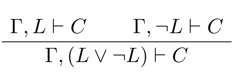
Formally, a lemma can be viewed as a logical cut. This says that given axioms \(\Gamma\) and a conjecture C, we call L a lemma if L can be proved from \(\Gamma\) and C can be proved from \(\Gamma\) and L. Recall that this turnsitle notation is used, so “\(\Gamma, L \vdash C\)” means that C can be proven from \(\Gamma\) and L. Written as a rule in a standard notation:

Wikipedia’s suggests the classic example where from “Socrates is a man” and “all men are mortal”, we judge that “Socrates is mortal.” Note that the fact that Socrates is a “man” is not in the conclusion as it was only instrumentally needed in the proof.

Automated theorem proving is generally done by looking for a refutation, so the proofs are actually of the form \(\Gamma, \neg C \vdash \bot\), from the axioms and the negated conjecture, we prove False (this bottom symbol, \(\bot\)). Therefore Josef used a hack with the law of excluded middle, “\(\Gamma, (L \vee \neg L) \vdash C\)”. Because “L or not L” always holds in classical logic, nothing is changed about the provability of C from \(\Gamma\). This allows the problem to be split into two in a slightly different manner:

In refutational form, the sub-problems look like: “\(\Gamma, L, \neg C \vdash \bot\)” and “\(\Gamma, \neg L, \neg C \vdash \bot\)”. We can consider the first sub-problem as the ‘negated conjecture’ form of the following, aiming to proove “not L” from the negated conjecture and the axioms, “\(\Gamma, \neg C \vdash \neg L\)”. Then this looks like the standard cut-rule where the goal is a contradiction (‘\(\bot\)’), the negated conjecture (\(\neg C\)) is one of the axioms, and the negated lemma is the cut (\(\neg L\)). Which gets to be a bit of a loopy brainfuck but it’s in some ways more aligned with refutational theorem proving (and it’s what was done =D).

(There’s another nitty-gritty technical reason for this formulation: something called Skolemization is part of the pre-processing step for dealing with first order formulas in a clause normal form and these skolem symbols from \(\neg C\) might appear in \(L\), which would be annoying to deal with when trying to prove “\(\Gamma \vdash L\)”.)

We define the proof shortening ratio (psr) as the following:

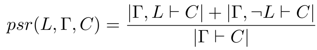
If E can prove both sub-problemmas in fewer given clause loops than E takes to prove the conjecture, then the proof ratio will be less than one and we judge that: L is a good lemma.

Of the 230,528 proof clauses, 98,472 of them are from the axioms or negated conjecture. There are 44,895 positive examples (including the 154 lemmas with a proof shortening ratio of 1) and 87,161 negative examples. The psr of most of the negative examples were not more than 2 — though I believe some went up into the 40s. (I did a bunch of fun statistical analyses that may not be revived 🤔 🤓.)

I believe this is a really cool way to measure whether a formula is a lemma: does the formula actually help one to prove the conjecutred theorem more effectively?

---

Dreamy Lemmata Desiderata

The dream is to generate (hypothesized) lemmas for a given set of axioms and conjecture. Heck, it’d be best if all known (mutually consistent) math could be considered as potential premises for a given conjecture and lemmas could be generated as stepping stones toward proof, ideally being theoretically evocative and meaningful, not just pragmatically useful. I think this is why the github repo for the dataset is called E_conj for E conjecturing.

If unable to do the above, maybe it’d at least be cool to look at an incomplete proof-search to identify clauses that seem promising (i.e., potential lemmata). The ENIGMA and ProofWatch systems I’ve worked on for guiding E thus far don’t learn from incomplete proof attempts — it’s hard to even identify what was done ‘wrong’ for negative reinforcement.

Colleagues have attempted this in a paper entitled, “Learning Theorem Proving Components“, tho I prefer the term Leapfrogging. The idea is to use a GNN (graph neural network) to do premise selection on processed or generated clauses (in addition to the original premises) to choose what to consider as a premise in the next run of the prover. Rinse and repeat. Maybe some generated clauses will actually be good premises. One technical challenge is reconstructing the proof (by refutation) after a few rounds of successive leapfrogging. An initial experiment on 28k hard Mizar problems found that leapfrogging can help E to prove hundreds of new problems.

The idea with theorem proving components is to cluster processed or generated clauses into related components to explore and then merge back together. Sometimes proofs can be split into distinct components that don’t have to be solved together, right?

For this project of mine, I just look at training classifiers or regressors to predict the proof shortening ratio of clauses, figuring if this is good, it could be helpful as a first step.

Lemma Classification

I used a scikit-learn to do a Singular Value Decomposition (SVD) of the 219,724 ENIGMA features. It turns out that the sdbm hashing is good enough even if the SVD has some theoretical merits.

I used scikit-learn’s Support Vector Machine (SVM) classifier, too. This technique is a generalization of finding a line to split data. What if this line is over some higher-dimensional space? If “\(x^2\)” and “\(y^2\)” are features, then a circle can be a linear separater 😜.

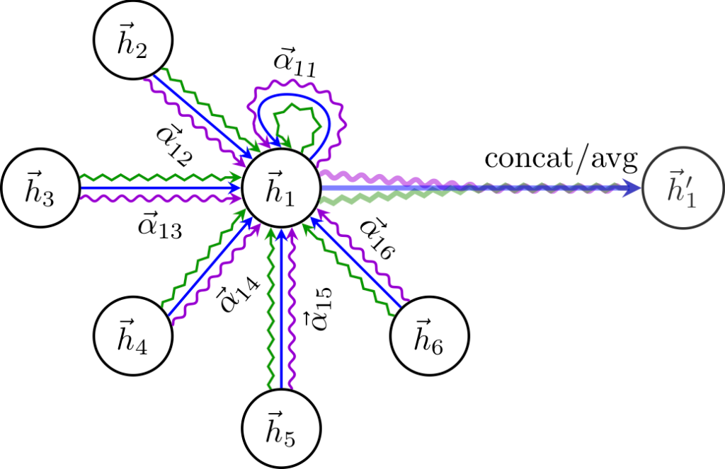
I wanted to try using some form of graph neural network and chose Graph Attention Networks (GATs) [arxiv]. In convolutional neural networks, one learns pixel features based on the neighboring pixels (which loosely mirrors what happens in the visual cortex). Enter graph convolutional networks: what if the features for a node in a graph are determined by the features of the node’s neighbors in the graph as in the image below where \(\vec{h}_1\) becomes \(\vec{h}_1’\)? The addition in the attention network is to add an attention function to calculate \(\vec{\alpha}_{ij}\) in terms of \((\vec{h}_i, \vec{h}_j)\) (– which is just a single-layer neural network followed by a softmax function in their work). With each layer of the graph attention network, the radius of influence on \(\vec{h}_1’\) increases by one.

How does a graph convolution relate to lemma identification?

Glad you asked!

Formulas can be represented as trees or graphs (when you take shared variables into account etc). Proofs are also directed acyclic graphs (though standardly depicted as sequences where each step is an axiom of follows from an inference rule from previous steps). Mathematical theories are dependency graphs (which Martin tried to use to guide Vampire’s clause selection via recursive neural networks, after this project of course 😂😁).

Maybe the graph structure of a proof can prove useful to help identify lemmas: for each clause L, what are its parents and children (and their ancestors)? by which inference rule was L derived? I found some fun schemes to encode the inference rules from E as edge weights in the grgaph. For the GAT, the proof graph is just an adjacency matrix whereas inference steps often include at least three nodes (two parents and one child), which should be represented as hyperedges.

The other catch is that formulas must be represented vectorially and how to do this is/was a burning research topic (which Mírek did a good job advancing and I’ll cover in the next post).

I also tried using XGBoost out of curiosity before presenting at AITP 2019. I was a very biased researcher, curious to play with a graph neural network and a believer in mind-world correspondence principles stipulating that the mental models should probably align with the structure of the data. However, hey, XGBoost was working pretty well for ENIGMA’s guiding given clause selection in E. The concatenation of clause and conjecture features is used for XGBoost and the SVM.

Results

I decided to primarily focus on how well the GAT and SVM predict good lemmas as the negative case seems less relevant. I recommend consulting the Wikipeida image on precision and recall (as I find the terms can be confusing):

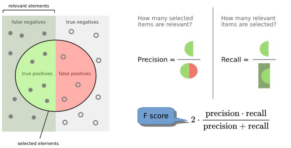
Recall is the accuracy on good lemmas and precision is the degree to which only good lemmas are classified as good. For the use-case of mining incomplete proof attempts, I’d wager that precision is the more important metric as we don’t want to waste time on false positives. The F-Score is a measure that combines precision and recall into one.

The GAT was trained with a strong bias toward precision on positive examples yet XGBoost crushes it with an all-around victory.

I think that XGBoost is probably good enough to try in the field:

1. Take a failed proof run.
2. Ask XGBoost if there any any good lemmas in the set of processed or generated clauses
3. Try to run ENIGMA over the two sub-problems.

This is very similar to the leapfrogging experiments.

The difference is that to train XGBoost in a mathematical domain, one needs to do an exhaustive evaluation of many proof clauses as lemmas.

Maybe someone will do it eventually (or future research will obviate the interest and utility of this avenue).

The slide shows from the AITP presentation and the short abstract are available for perusal.